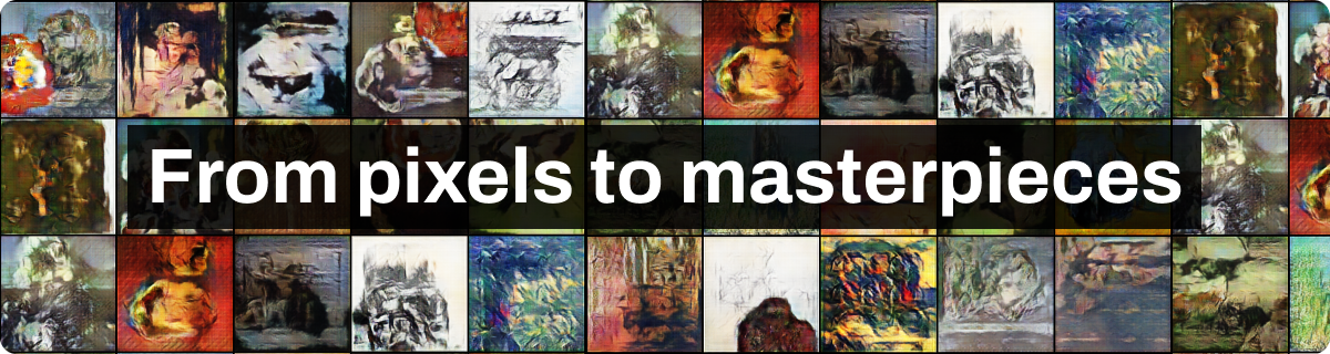
From Pixels to Masterpieces, My journey of building a generative AI model from scratch

As part of my internship challenge at Rootcode AI, I got the opportunity to build an AI model that can generate artwork, and I'm excited to share my experience building it. In this article, I will delve into the fascinating world of AI and show you how generative models can create beautiful and intricate artwork. Discover how machines are becoming more creative than ever before and what this means for the future of art and technology. So, buckle up and get ready for a mind-bending journey into the world of machine creativity.

What is Project Artistry?

During my first week, I was presented with an internship challenge. We called this “Project Artistry”. This challenge involved using Artificial Intelligence to generate stunning art. What made this challenge particularly intriguing was the impressive dataset of approximately 8000 digitalized artworks, crafted by 46 talented artists, that I was given to work with.

Since generative AI was a new topic for me, I started by reading about generative models and their applications. Generative AI is a subfield of AI that focuses on embedding human-like creativity into AI models to generate content. And these AI models are capable of generating content that is similar in style and quality to existing examples without generating an exact copy, consequently simulating the idea of embedding creativity in its generative mechanisms.

When I did my research on generative models, I came across Generative Adversarial Networks (GAN), which is a type of neural network architecture invented by Ian Goodfellow in 2014. The simple idea behind GANs is to train a neural network on a dataset and use the patterns learned by the neural network to generate data items similar to the items in the dataset using the learned patterns. For example, if we train a Generative Adversarial Network on a dataset consisting of paragraphs of poetry, it would use the learned linguistic structures and patterns from the dataset to generate its own form of poetry, which would embed the same patterns in the dataset.

Training a Generative Adversarial Network

This is done by training two neural networks; a generator, and a discriminator, in a two-part process:

• The generator network produces new data samples, which are then fed to the discriminator network.
• The discriminator network tries to distinguish the real data (original data) from the fake data (generated data) produced by the generator.

Confusing?

Credits: Mayank Vadsola (source)

Let’s assume the generator is a counterfeiter who prints money and the discriminator is a police officer who has to distinguish between real and fake money. In the beginning, the counterfeiter is trying to print some money that looks like pathetic forgeries because he hasn’t yet learned what real money should look like. The police officer is then shown the real money and the fake money, and he tries to guess whether each of them is real or not. His guesses might not be good at this point. But the police officer gets to know the true label of each money. That is, whether they are real or fake.

Using these labels, he understands how to identify which is real and which is fake with time. For example, He gradually improves his knowledge, like if it has a value at the corner, it might be real, and so on. He is also encouraged to learn as he is penalized for distinguishing each time incorrectly. The counterfeiter also then learns to create better forgeries to fool the police officer.

This then continues when both of them try to improve their capacity in their work. The Counterfeiter tries to print fake money that is indistinguishable for the police officer, and the police officer tries to distinguish between real and fake money correctly. Both these individuals are in a minimax game, trying to minimize their losses and win the game.

Can we use a similar idea to build an artwork generator that can generate similar artworks similar to the art done by famous artists such as Picasso, Giotto, Rembrandt, etc? Well, to do that, I would need their artwork for that right? Fortunately, my dataset consists of their artworks and contains a variety of artistic styles as well. Below are some examples of the original artworks I used. The artworks fall into still life, landscape, seascape, portraiture, and abstract styles. From here onwards, let’s try to build a generator that has learned to draw real-looking artworks.

Figure: A sample of the original artwork

Let’s Build our Model.

If you can remember, the entire architecture should consist of a generator and a discriminator. The generator learns to create real-looking artwork, and the discriminator learns to distinguish between real and generated artwork. Consequently, both the generator and discriminator get better, and the learning stops once the generator successfully fools the discriminator into thinking that the generated images are real.

First, let’s see how to build the generator from scratch

Figure: Input and output of a generative model The generator takes in a random noise input and uses this to generate a synthetic data sample, such as an image or a piece of text. The structure of the generator network can vary, but it typically consists of a series of layers that learns to construct images from noise. The generator is typically trained using an optimization algorithm, such as stochastic gradient descent, to minimize a loss function that measures the difference between the generated samples and the real samples. The optimization algorithm here tries to find the best values for the parameters (such as weights and bias) in our neural network to generate real-looking samples.

In simple words, the generator is trained towards reducing the difference between generated samples and real samples using optimizers. When the difference is smaller, the generated artworks look like real artworks.

I started the generator with all the dense layers and observed that it was really bad at generating images similar to the real images after training. So I decided to move forward by using Convolutional Transpose Layers.

Why Convolutional Transpose Layers?

Convolutional Transpose Layers are also a type of layers used in Convolutional Neural Networks. Convolutional layers are designed for detecting features of an image, but transposed layers can upsample an existing image by increasing the spatial resolution of the feature maps. We can even think that convolutional transpose layers do the reverse of convolutional layers. The convolutional transpose layers are mostly used in generation tasks. Simply these layers can map lower-dimensional feature maps to higher-dimensional feature maps, enabling the output of higher-resolution images.

Figure: This is the generator architecture I used

Now let’s see how we can build the discriminator

The role of the discriminator is to identify whether a given data is real or fake. This means that the discriminator is simply a binary classifier. It needs labeled data to learn whether it has identified the label correctly. That means we have to label all the outputs from the generator as fake images and all the images from the real data set (our training dataset) as real images. We then shuffle these images and provide those as input to the discriminator.

Figure: Generator and Discriminator Source: Source

The structure of the discriminator network can vary, but it typically consists of a series of layers that extracts features from the input data and uses these features to make a prediction on whether the input data is real or fake. During training, the generator and discriminator are trained together, with the generator trying to produce fake images similar to the real artworks in our training dataset to fool the discriminator and the discriminator trying to identify whether each data sample is real or fake accurately.

Figure: This is the discriminator architecture I used.

To entropy or not entropy?

Previously I mentioned that our generator and discriminator are a type of neural network each with a different learning goal. Each of these neural networks has its parameters such as weights and biases that the model learns to achieve its learning goal. Mathematically, this is guided by a loss function that informs the outcome of the model’s learning. From the results of the location, it learns to improve the estimation of its model parameters. Therefore, I need a loss function to learn the model parameters. In my challenge, I initially started with Binary Cross Entropy Loss but after evaluating the training process and results, I observed a drawback in using this loss function. Therefore, I did some more reading and implemented another loss function which gave me some desirable results. Let’s discuss them one by one.

What is Binary Cross Entropy Loss?

Binary Cross Entropy Loss(BCE) is a loss function used in GANs to measure the difference between the predicted probability of a binary event (e.g. real vs fake image) and its ground truth label. In a GAN, the generator model outputs an image, and the discriminator model outputs a prediction on whether the image is real or fake. The Binary Cross Entropy loss is then used to calculate the difference between the predicted probability of the image is real and the ground truth label (1 for real, 0 for fake). The objective of the training is to minimize the loss function to improve the discriminator's ability to classify real and fake samples correctly

BCE loss = -E(y *log⁡(p))+ E((1-y)*log(1-p))

Where,

• y = Ground truth label (1 for real, 0 for fake)
• p = Predicted probability of the image being real

What are the problems with Binary Cross Entropy Loss?

My dataset consists of artworks from 46 artists and is a mix of various artistic styles and color mixings. But when I observed the images I generated using the Binary Cross Entropy loss, it looked like it generated images of some particular style only. When I was trying to find out why there was no diversity in the images generated, I realized it is a popular issue in GAN which is called mode collapse. To understand what mode collapse is, let’s first briefly look at what a mode is. Mode is the higher-density area which is usually signified as a peak in the distribution. The mode contains a concentration of the highest number of similar occurrences. In the real world, most of the distributions have more than one mode (multimodal) – similar to the figure given below. In this problem, we should have multiple modes for different artistic styles;, not only that, we have to replicate that distribution using the GANs to generate diverse images.

The Binary Cross entropy loss compares the generated image’s prediction with the actual label (real or fake), then adjusts parameters. Once the generator realizes that it fooled the discriminator by a few samples, then Binary Cross entropy loss becomes stable, and the gradients will become small, making it difficult for the optimizer to update the model's parameters, leading to mode collapse. That means the diversity of generated images becomes poor.

This will end the learning process, which means converging into a sub-optimal solution (which means getting stuck at a few particular styles), not a global-optimal solution.

Figure: Sample output while training with BCE: Trying to generate the same styles

To find a solution to this problem, I collaborated with my team to brainstorm potential solutions. During these discussions, I had an exciting breakthrough idea: what if we could penalize the difference between the real and generated distributions more robustly to achieve a more stable training process and prevent mode collapse? And that’s where Wasserstein Loss came into play.

What is Wasserstein's loss?

Imagine that you have two piles of hay, as observed in the figure. Let’s name these piles X, and Y. Let X be the predicted distribution of the data, and Y be the true distribution of data. To make X look like Y, you have to re-arrange the haystack. This is where Wasserstein loss (W-loss) comes in. The W-loss calculates the minimum amount of hay that needs to be moved to rearrange the X pile to look like Y. This is why Wasserstein loss is also known as the Earth Mover’s Distance.

To recap, for our image generation task, the GAN model’s generated distribution(X) should be like the real data distribution(Y). Unlike the traditional Binary Cross entropy loss, W-loss evaluates the performance of a GAN generator by calculating the Earth Mover's Distance between the generated and real data distributions, making it more stable and easier to optimize than traditional loss functions.

We know that a distribution has its own properties such as skewness, mode, etc. GANs should learn to replicate the real-world distribution, including its properties in their learning parameters. Therefore, it is necessary to have a suitable way of measuring the difference between replicated distribution vs real distribution. W-loss that measures the distance between two probability distributions might be a good solution.

Moreover, W-loss is independent of the different properties each distribution has. To recall, it only measures the minimum amount of work to transform one to another. This means from here onwards, we don’t need to worry about mode collapse.

Importantly, the discriminator is no longer discriminating against the inputs to determine whether they are fake or real. Now it describes the difference between real and fake images and helps the model learn. Therefore we can call it the Critic from here onwards. Because unlike the discriminator, a critic would not only tell whether the image is fake or real in a binary output but would also give a probability distribution on how “bad” the fake image is.

Therefore, I can see that choosing the correct loss functions is one of the crucial parts of the training. Additionally, the W-loss has several advantages over the Binary Cross Entropy loss. For example, it is smoother and easier to optimize, which can lead to more stable training and better results. It is also less sensitive to the choice of hyperparameters and has a more intuitive interpretation in terms of the distance between the real and fake data distributions.

Let’s add them all together and see

We now have the model for our generator, discriminator, and our loss function. The training process is based on a few simple steps. But here, the most important thing is we cannot train both Critic(Discriminator) and the Generator simultaneously. It is like hitting a moving target, while we are also moving. It is not possible in neural networks, especially when the generator needs the discriminator’s feedback to update the learning parameters to generate more realistic images.

So here what we do is;

• First, we need an input for our generator network. Therefore, we will input a batch of random noise into the generator.
• Then the Generator outputs a batch of fake images.
• The next step is where the Critic is trained. We have real artworks which are also labeled as real. We will mix those real images with the fake images for the Critic. Then according to the critic loss, the weights are adjusted only in the Critic.
• To train the generator, we create a batch of fake data and label it as real. We then pass this fake data through the critic and use its response to update the weights of the generator – The goal is to improve the generator's ability to create more realistic data by adjusting its weights based on the feedback from the critic.
• So now we have completed one iteration in our GAN training. We can let the process run iteratively to a large number of epochs to get a well-trained Generator.

Figure: Overall process of learning the parameters

Here is what our generator can do

After a few iterations, we can see the Generator has started to generate some images that contain different styles, colors, etc. It is a signal that the model is learning. Earlier, our generator was similar to a small kid who started drawing without any knowledge about arts such as colors, structures, and styles. Initially, the generator’s drawings got rejected as they were not good enough to fool the critic into thinking real artists drew them. Then using those feedback, the generator continues to improve its generated images, and after a lot of paintings now, the generator is capable of applying the shades, structures, and patterns to everything like Picasso, Giotto, Rembrandt, etc.

We can save the Generator model separately, which now behaves like an artist with some skills to sketch real-looking artwork.

Figure: A sample of generated outputs

How to evaluate the generated artwork?

In machine learning, it is crucial to analyze models to verify whether they have learnt generalizable patterns from the dataset. This is where evaluation comes in. We evaluate the output of a machine learning model to check how well the model has performed.

If we are generating real objects like faces, fashion items, etc., we can use pre-trained classifiers, which were trained on millions of images. Once we remove the final layer, we can come up with all the features for a given input image. So we can use those features as a measure of reality and compare them with images generated by our generator.

But unlike real-world objects, artworks are basically abstract images. Additionally, artistic abstraction, representation, freedom, and creativity mean that it is not always necessary to create an object or any real-world representation in the artwork; it could be a mixture of different colors, some pencil lines, or anything. This means that the way it is perceived depends on individuals.

So how can I evaluate whether the generated images look like real artwork? That is where I thought the best way to get started is by inspecting them with the human eye, whether these artworks look real or not to a human. That's how I could understand whether the model is learning and the quality and diversity of artworks in the training dataset.

Wrap-up

After spending a few weeks with GANs, building the architecture, training the models, tuning the hyperparameters, and conducting many experiments, the challenge came to an end. I shared my overall experience with the team by presenting the results and thoughts to the team. Generative AI is definitely a fascinating topic, so having this kind of experience to learn and enjoy during my internship was satisfying.

Figure: A sample of generated outputs

You can check out my implementation in our open-source repository: RootcodeAI-Intern-Challenges

References

• Goodfellow, I., Pouget-Abadie, J., Mirza, M., Xu, B., Warde-Farley, D., Ozair, S., Courville, A. and Bengio, Y. (2020). Generative adversarial networks. Communications of the ACM, 63(11), pp.139–144. doi:10.1145/3422622. https://arxiv.org/pdf/1406.2661.pdf
• Gulrajani, I., Ahmed, F., Arjovsky, M., Dumoulin, V. and Courville, A.C. (2017). Improved Training of Wasserstein GANs. Neural Information Processing Systems
• Radford, A., Metz, L. and Chintala, S. (2015). Unsupervised Representation Learning with Deep Convolutional Generative Adversarial Networks. arXiv.org